BG Deep Science: Hidden Dynamic Inference Based on Neural Manifolds

Hi guys, today let’s talk about using deep learning methods to infer the hidden dynamics in the neural process based on neural manifolds. I’m going to give you brief introductions to three models: LFADS, NoMAD, and DFINE. I’m also going to talk a little bit about my current work, Meta-KF.

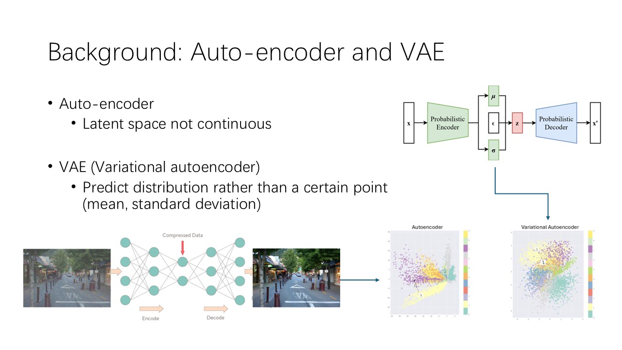
Let me first give you some background introductions. Last time in Deep Science, Carlos had already introduced autoencoders to us. Basically, as you can see from the plot below, an auto-encoder is trying to compress the data and express the data using fewer features. The two-neuron layer is called the bottleneck of the auto-encoder, where the model uses these two values to express the 4-feature input data, and also reconstructs it back to the 4-feature data again.

The problem with traditional autoencoders is that the latent space is not continuous, and they overfit significantly to the training data. As you can see from the plot on the right, even though the points are clustered well, the distribution is not continuous, so when you sample the middle point of a plot of number 1 and plot of number 2, the reconstructed plot is very likely to be a non-sense.

To stress this, variational auto-encoders were invented. Instead of mapping the raw data to a point in the latent space, the VAE maps the raw data to a distribution in the latent space by learning the mean and variance of the distribution, as you can see on the right. The main idea here is that when you sample a point in the latent space close to plot 1, the closer the point is, the more the reconstructed point should look like the plot of number 1.

Therefore, the latent space is now continuous, and if you sample the middle point between the plot of 1 and the plot of 2 here, you will get a reconstructed plot looks like something in between.

Now, the second thing I want to introduce is the State-space model. We are all familiar with the Kalman filter, which is based on State-space models.

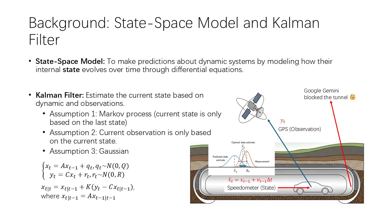
State-space model is used to make predictions about dynamic systems by modeling how their internal state evolves over time through differential equations.

I will give you a very simple example. Imagine driving a car through the tunnel. How do you know where exactly you are in the tunnel? There are two things you can use. The first one is the GPS; at every timestep, your car is sending your location to the satellite. But this is not accurate because you are in a tunnel and the signal is weak. The second thing is the speedometer on your car; you can use your speed to calculate how far you just went.

The GPS is called observation, and the speed of your car is the dynamic of your car, which is the first-order differential equation of your location, which is the state you want to infer. Neither of these is 100 percent accurate; they all give you an expectation and their uncertainty, which forms a distribution. And you can use the Kalman filter to combine these two distributions to get a more accurate and certain result.

Here’s the equation of the Kalman filter: your current state estimate is a transition matrix A times your last state plus a zero-mean Gaussian noise, which obeys assumption 1 that this is a Markov process. The second equation means that your current observation is an observation matrix C times your current state plus a zero-mean Gaussian noise.

Here, your optimal current estimation is a weighted sum of your state estimation based on the dynamics and observations.

As you can observe in the equations, all these processes are linear and Gaussian. Therefore, all the parameters can be fit using the least squares method.

In our scenario, the state is the cursor kinematics, and the observation is the neural signal we are recording.

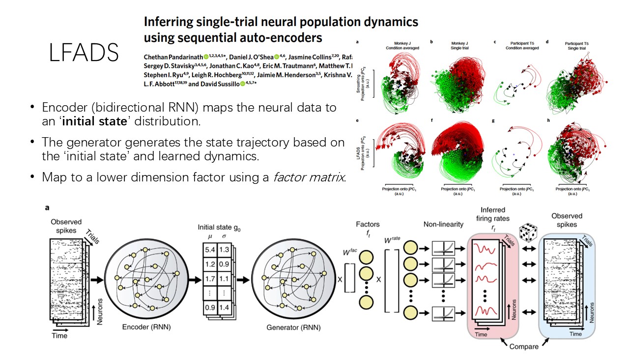
Let’s talk about Chethan’s LFADS model. LFADS is also an auto-encoder model, but for sequence data like neural data. The most important components in LFADS are the two RNNs, the encoder and the generator.

The encoder is a bidirectional RNN that maps the neural data to an initial state distribution. For each trial, the input to the encoder is two-dimensional, which is time and features, and the output will also be two-dimensional, which is 2 and the number of features. The first column is the mean of the distribution, and the second column is the variance.

The initial state distributions are then input into the generator, which generates the sequence again from the initial states and learned dynamics.

After re-generating the sequence, a factor matrix W_factor is used to linearly reduce the dimensionality and extract the factors. To reconstruct from the factors, another matrix W_rate was applied, and also exponential functions to ensure non-negativity.

As the jPCA figure in the upper-right corner shows, the LFADS regenerated neural trajectories are more consistent and less noisy on both monkey and human data.

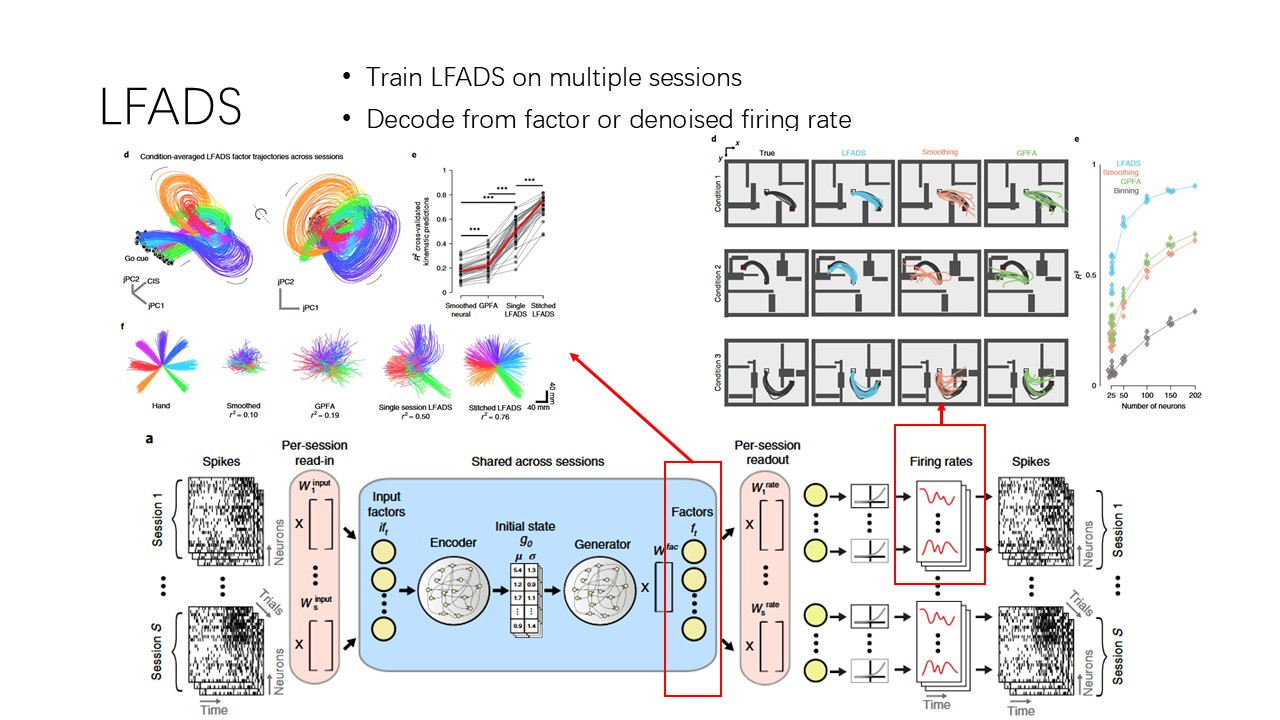
Chethan also tried to train LFADS using multiple sessions. A linear input matrix and readout matrix were trained to align the data from different sessions. This can also be considered as a day layer.

To decode the behavior data, the LFADS paper used the inferred firing rate for single-session decoding and factors for multi-session decoding. The firing rate decoding result from a monkey maze task is shown on the left, and the multi-session result is shown on the right.

You can see from the figures that LFADS de-noised firing rate and factors have very good behavior decoding abilities.

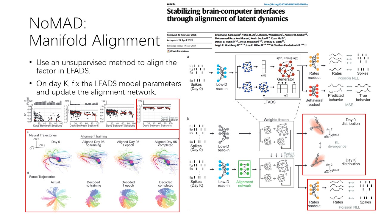
Now, after we learned about LFADS, let’s look at a new model just published based on LFADS from Emory. The model NoMAD uses LFADS to infer the neural dynamics of the neural data from different sessions. The main idea is to use another alignment network to align the LFADS inferred neural dynamics on day 0 and day K, and then decode using the behavior decoder trained on day 0.

The LFADS model is fixed and no longer updates after day 0 when it was first trained. On day K, only the read-in network and an alignment network were trained. To make sure the distribution of neural dynamics on day 0 and day K is aligned, the model needs to minimize the KL divergence between the factor distribution on day 0 and day K, while also minimizing the reconstruction loss on day K.

As you can see on the left, after the alignment training, the NoMADs showed the best decoding accuracy using the decoder trained on day 0.

You may also notice that the LFADS structure shown here is slightly different from the LFADS structure I showed in the previous slides. This is because there is another controller model feeding external inputs into the generator to better model the neural dynamics. This is explained in the LFADS paper; I won’t talk about it today, but please feel free to discuss with me later if you are interested.

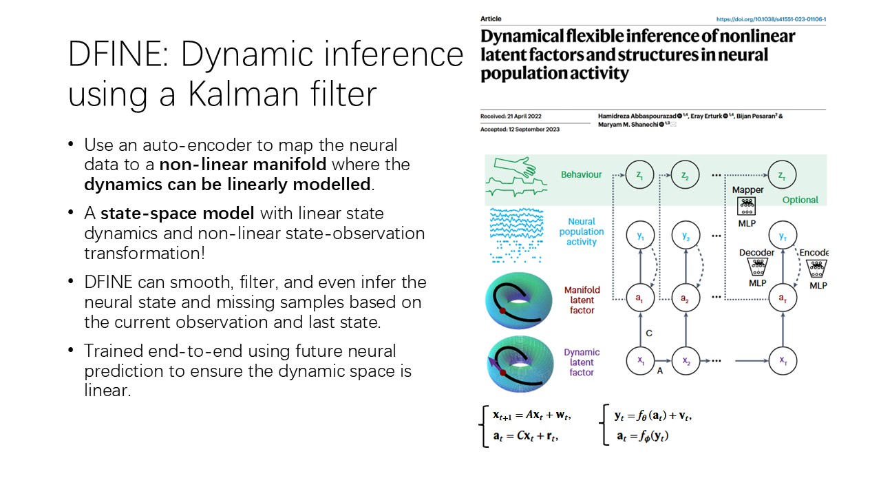
We introduced the LFADS to infer the neural dynamics using the RNN generator model. Here’s another model called DFINE, designed by Maryam’s lab, which uses a linear dynamic function, a Kalman filter, to model the neural dynamics.

The main idea of DFINE is to use an auto-encoder to map the neural data to a non-linear manifold where the dynamics can be linearly modelled. It can be considered as a state-space model with linear state dynamics and a non-linear state-observation transformation. The equation on the right is the dynamic function of the DFINE model; f_theta and f_phi are the encoder and decoder.

Looking at the plot, the neural data y can be transformed to manifold factor a, which is this non-linear donut. The dynamic factor x is linear on this donut manifold. To understand this, you can think about Ruixiang’s spherical cursor. Even though the participant sees the cursor going through a curve on the 2D monitor plane, the cursor is actually going through a straight line on the sphere.

The dynamic factor here is linear, so the transition matrix A and observation matrix C are the same as the state-space parameters A, C we saw earlier. Dynamic x is the inner state, while manifold factor a is the observation.

The DFINE model is trained end-to-end, and even the dynamic factors A and C are fit using gradient descent methods together with the auto-encoder to make sure the dynamic system is linear.

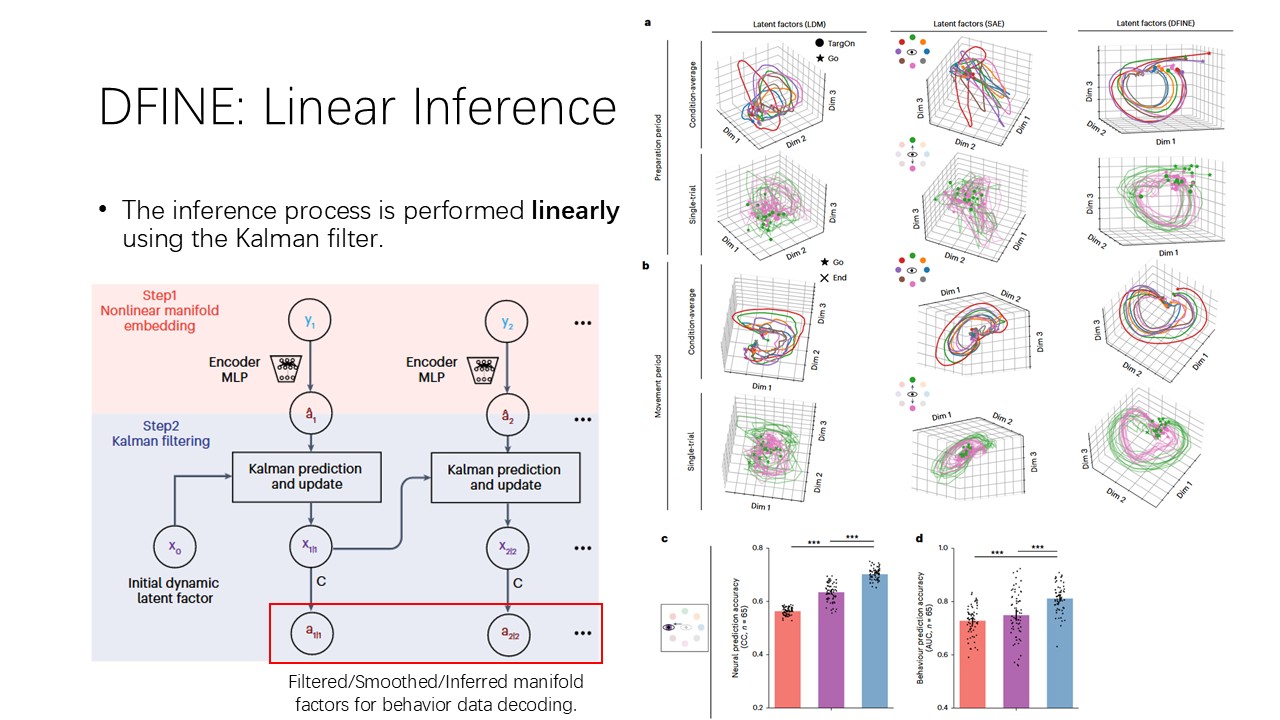
The inference, filter, and smooth processes are all linear in the DFINE model by using the Kalman Filter, which makes DFINE require much less computing resource to infer data.

As you can see on the left, for real-time filtering or inferring, when a new neural observation sample comes in, the manifold factor a_t can be inferred using the encoder. This manifold observation a_t is used to estimate the current state x_t together with the last state x_(t-1).

The manifold factor a is used to decode the behavior data or calculate the neural trajectories. You can see in the right figures, the DFINE gives even better accuracy compared with a linear dynamic model and even LFADS, which is called SAE here.

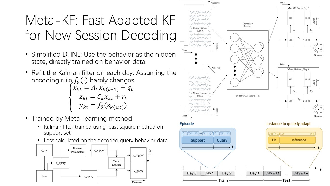
After learning all these models, I want to talk about my current work, Meta-KF. This work can be understood from two points of view: the meta-learning POV and the neural manifold state-space model POV. I will mainly talk about the latter one because this is the topic today.

Meta-KF can be considered as a simplified version of DFINE. Instead of decoding the behavior data from dynamic factors, the Meta-KF model takes behavior kinematics as the internal state x.

The assumption is that there is an encoding rule that barely changes to non-linearly map the neural representation of the behavior to the neural space, while in this neural representation manifold, the behavior dynamics are linear.

The model structure is shown on the right. On each day, we put the neural data into the model learner, which acts as the encoder in the DFINE paper. The learner can be any model; in my work, I tested both an LSTM model and a transformer model as the learner. The learner here, which is the f_theta in the equation, maps the neural data to a learned stable low-D neural manifold. A Kalman filter is then trained on the low-D manifold data, since the manifold is optimized to fit the Kalman filter and express the dynamics linearly, the new Kalman filter can be fit using only a few trials. Furthermore, because the Kalman filter here is fit using the least squares method, the updating process is much faster than training a new network.

The learner pre-training is based on the meta-learning method. As illustrated on the right, the training data is split into small segments called episodes. Each episode is then split into a support set and a query set. The support set is first fed into the learner to get the low-d support data, then the Kalman filter will be fit on the low-d support data. After fitting the Kalman filter, the model will decode the behavior data from the query set and calculate the loss to update the model. The gradient flow is shown in the plot below.